MajorFault.io

So I've been meaning to keep this post for a project I have in my head, but I'm too excited.

Let's talk about PID tuning.

Often, PIDs are simply tuned "by hand" without much regard to the dynamics behind the principle. I think that for most people, it is an arcane art. I happen, for some reason, to really enjoy the theory behind continuous control, and the project I'm working on is a way to both demystify this and also make it easier.

For now I have the numerical analyzer working - the rest of the project will be to integrate it into my website in the form of an engine that people can submit their trend data to. It then spits out a model and recommended parameters and plots them. So let us explore this piece of the puzzle: this will be able the "system identification" part of the feature.

The first order plus dead time model

Most process responses can be modelled using three components:

• An amplifier
• A low pass filter
• A delayer

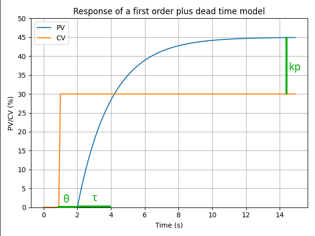
The amplifier (kp, unitless) reflects the difference of scale between the action of the CV and the reaction of the PV. For example, if I make my pump go 10% faster over its possible RPM range, I might only get 5% more flow over the instrument range. If we look at this using percentages of scale, the action is amplified by 5 / 10 = 0.5. This would correspond to a process gain of 0.5.

The low pass filter (τ, seconds) damps the high frequency components of the reaction such as that the reaction looks like an exponential function over time. This can be due to many things: the characteristics of the process, the instrumentation reaction time, and so on. There is rarely only one source of lag, however we can subsume them all into one and stay relatively accurate. The value of τ is the time it takes for the reaction to reach 63.2% of its total change, after dead time. The higher τ is, the more sluggish the process is.

The delayer (θ, seconds) is simply the physical delay between the action and the start of the reaction. For example, imagine dumping rocks onto a conveyor belt. A scale placed at the end of the conveyor belt will not read the added weight until the rocks reach it. From the point of view of the scale, the belt might be empty even if rocks were just dumped onto it. If we look only at the scale, we might be tempted to add more rocks! This is why that as θ gets proportionally bigger, processes get harder and harder to control.

The combination of the effects of the amplifier (process gain), low pass filter (process lag) and the delayer (process dead time) can be modelized as a first order (one lag - higher order models exist) exponential model, plus the dead time.

Using the variable y as the process output (the PV), u as the process input (the CV) and t as the time, we can express this relationship with the following differential equation:

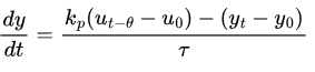
This is called a first order plus dead time model. The model looks like this:

Optimization

Optimization is the mathematical process of adjusting the parameters of a function until its return value is minimized or maximized. In other words, there could be a way to take this equation above, and to modify the values of the three parameters kp, τ, θ up until it takes a minimal or maximal value. How can we use this to our advantage?

Let's imagine that we have a trend of our process loop. We have trended the PV and the CV with regards to time, whilst turning off any existing controller. We may have put the loop in manual mode and simply moved the actuator up and down to register the process values. This is called open-loop testing, and these are our empirical results. If only we knew the values of kp, τ, θ, we would be able to calculate the PV at any time on our graph. Unfortunately, processes don't come with these values...

This is where optimization can help us. What if we took our model, entered some set of parameters, and used it to compute a PV, given the time and the CV value that we can find on our trend? We could then calculate the difference between the model estimation and the real value on the trend, and find out how far we are from the real value. Then we can try another set of parameters, and find out if this difference has increased or decreased. This way, we can know if we're playing with the parameters in the right or the wrong direction. Do that a bunch of times over all the values on the graph, and we will eventually find a set of parameters that causes the PV values of our model to be closest to that of the trend.

Fortunately, computers can help us with this! Let us define the sum of squared errors (SSE) as the squared difference of the trend PV (y) and the model PV (y-hat) over the time span:

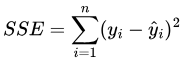
SEE has been chosen for two reasons:

• We don't care about the polarity of the error. A positive or negative error is an error! We only care about its magnitude.
• Squaring the error penalizes large deviations more strongly than small deviations. We don't want to get lost trying to fit noise (which is an irreducible error).

Then what we're looking to optimize is simply min(SSE). If we can get this error to as close as zero as possible, we should be able to get reasonable approximates for kp, τ, θ that will allow us to calculate our PID gains with accuracy.

This is called system identification.

System identification in code

I have been playing around with Julia, a language expressly made for scientific computing. The following code will be in Julia, using the DifferentialEquations, Optimization, OptimizationOptimJL, OptimizationBBO, Interpolations and CSV packages. You can find the full code at this GitHub link. Feel free to try it out (I know - I don't have a readme. Sorry :( ).

First, let's define the model equation:

function first_order!(dy, y, p, t)
    u_delayed = t < p.θ ? p.bias_u : p.interpolated_u(t - p.θ)
    dy[1] = (p.kp * (u_delayed - p.bias_u) -(y[1] - p.bias_y)) / p.τ
end

This is simply the equation I've written above. The first order plus dead time model is not an ordinary differential equation: it's a delayed differential equation. We can shift it to an ODE that's easier to solve by using the following trick: clamp the CV to its bias value if t < θ, else grab a time-shifted t - θ CV. This makes it so from the point of view of the equation, the dead time is effectively removed. This will allow us to use the simpler and faster ODE solvers. The in-place version (so-called because it modifies the array dy instead of returning a result) is faster.

We can do use this to calculate our model over the time span of the trend:

function generate_model(diff_function!, p)
    ode_problem = ODEProblem(diff_function!, [p.bias_y], p.t_span, p)
    return solve(ode_problem; abstol=10e-6, reltol=10e-6)
end

This code takes an in-place function and uses an ODE solver to compute the values of y over the time span. The sweet thing with the Julia packages is that they will automatically choose a suitable solver in order to calculate the result with the best accuracy. abstol and reltol are parameters that allow to tweak the accuracy of the solver when facing large values or near-zero, respectively. They are probably too low for this application but it doesn't really hurt.

Next, we need to calculate the SSE:

function calculate_model_sse(model, data)
    if SciMLBase.successful_retcode(model)
        model_y = model.(data.sampled_t; idxs=1)
        return sum((model_y .- data.sampled_y) .^ 2)
    end

    error("DiffEq solver has failed with code " * model.retcode)
end

Another neat thing with Julia is that it can broadcast operations in order to very quickly do them over a large data range. In this code snippet, .- and .^ are broadcast operators for subtraction and exponent.

Now to tie this all together:

function loss_function(parameter_vector, data)
    model_parameters = (
        kp = parameter_vector[1],
        τ = parameter_vector[2],
        θ = parameter_vector[3]
    )

    model = generate_model(first_order!, merge(model_parameters, data))
    error = calculate_model_sse(model, data)
    return error
end

This function exists because the optimization functions expect certain signatures. We haven't even started doing anything yet, but now we will. First we need to actually obtain the data from the trend:

function set_up_data(file_path)
    file = CSV.read(open(file_path), DataFrame; header=false)
    return (
        sampled_t = file.Column1 .- file.Column1[1],
        sampled_u = file.Column2,
        interpolated_u = linear_interpolation(file.Column1, file.Column2, extrapolation_bc=Line()),
        sampled_y = file.Column3,
        bias_y = file.Column3[1],
        bias_u = file.Column2[1],
        t_span = (0.0, file.Column1[end])
    )
end

I'm setting up a few things here. First, obviously, reading from the CSV. It does have to be in a very particular format: first column is time in seconds (and not timestamps), second column is CV, and third column is PV. So if you've got a sample time of 100 ms, the time column would look like [0, 0.1, 0.2, 0.3, ...]. I'm planning on making this a bit more robust for the final product, but this suffices to explain the concept.

For the sampled times I'm straight away subtracting the earliest time from all of them so the data set starts at 0. For the CV, I am not using the values of the trend directly, because they will be sampled and thus will have holes. ODE solvers usually use variable step lengths and we don't want our model function to crash out because the solver tried a time it didn't know about. So we'll take all the CV samples and draw a line through them. The solver will then be able to take arbitrary steps.

And finally we can start optimizing:

function optimize_model(file_path)
    data = set_up_data(file_path)

    initial_vector = [1.0, 1.0, 1.0]
    lower_bounds = [-200.0, 0.0, 0.0]
    upper_bounds = [200.0, 200.0, 200.0]

    black_box_function = OptimizationFunction(loss_function)
    black_box_problem = OptimizationProblem(black_box_function, initial_vector, data; lb=lower_bounds, ub=upper_bounds)
    black_box_solution = solve(black_box_problem, BBO_adaptive_de_rand_1_bin_radiuslimited())

    refined_function = OptimizationFunction(loss_function, ADTypes.AutoForwardDiff())
    refined_problem = OptimizationProblem(refined_function, black_box_solution.minimizer, data; lb=lower_bounds, ub=upper_bounds)
    results = solve(refined_problem, BFGS())

    strategy = recommend_strategy(results.u[2], results.u[3])

    return (
        residual_error = results.objective,
        kp = results.u[1],
        τ = results.u[2],
        θ = results.u[3],
        recommended_strategy = strategy
    )
end

For an optimizer to start...optimizing, it needs to start somewhere, so I've given it arbitrary guesses as a starting point. The closer the guesses are to reality, the more accurate the end model will be and the faster it will be computed. We could input them, but honestly I'm lazy. Also, I've always had decent results just putting in whatever.

The first optimizer we will use is a black box method, and it's bounded. What this means that the algorithm will only attempt kp, τ, θ values in the given range. Because it's physically impossible for τ and θ to be negative, this is a pretty nifty feature. The advantage of running a black box first is that these are global optimizers. If you remember your calculus classes, functions have global and local extrema (minima and maxima) - relative and absolute points where their values are lowest or highest. Black box optimizers are able to look for the global minimum of our SSE function without getting trapped into any local minimum that might exist. We'll run that one first to get in the right neighbourhood, then a local optimizer to refine the search in case our black box didn't find it itself. As for the AutoForwardDiff, this is because BFGS uses a gradient for its algorithm: we would need to provide it, but Julia can auto-compute it!

Last thing we do is recommend a control strategy with this function:

function recommend_strategy(τ, θ)
    if θ <= 0
        error("θ cannot be 0.") # avoid div by zero
    end

    ratio = τ / θ

    if 1 >= ratio
        return Advanced
    elseif ratio <= 2
        return PID
    elseif ratio <= 5
        return PI
    else
        return P
    end
end

The τ/θ ratio is a nice, quick and dirty way of judging the controllability of our process. Basically, θ is our biggest enemy. As θ approaches the value of τ, the dead time tends to overwhelm the dynamics such that simple PID control gets very hard. It's not hard to imagine why: there is a sizable amount of time where the PID algorithm tries to wind up or down the actuator without seeing the effects. In this case, a PID+ strategy is needed, for example a Smith predictor to modelize the process without the dead time. As the ratio gets higher, the control strategies we can use successfully get simpler and simpler.

A little test

I have a little .csv file where I've estimated the values of PV and CV for a process with parameters kp = 0.3, τ = 5, θ = 2. Let's see what happens if we try to analyze it:

As we can see, we get very close. It gets the gain down exactly, with tiny errors for the lag and dead time.

Following up

With these parameters in hand, we can use any one PID tuning method (Ziegler-Nichols, Cohen-Coon, Skogestad) to calculate PID values. It's simply algebra from there. Other interesting things to do:

• Plot the error term to find out how it looks. It should look like random noise. That is the irreducible error: the part we cannot fit to our model.
• Backfeed the parameters into a function that generates responses given PID tunings so we can have an idea of how the tuning looks.

Conclusion

The goal of this exercise was not to give a long course in controls theory but build a bit of intuition about how we might go around analyzing processes behind the scenes. I hope this has been a worthwhile read!